Dyadic or two person psychophysiology data includes nesting at three levels. First we have repeated measures nested within individuals. Next we have individuals nested within dyads. When considering modeling how measures of interest at the individual level (i.e. personality) or at the dyadic level (i.e. relationship satisfaction) may relate to individual differences in a physiological response it is first important to consider if we have ample variation at the within-individual, within-dyadic, or between-dyad level. Investigation of the amount of variance in physiology related to these different levels can be accomplished by calculating intra-class correlation (ICCs) or the proportion of variance attributed to our level of interest. Calculation of ICCs can be readily computed in a Bayesian framework which assumes normal distributions for our psychophysiology data at the three levels.
For this example, I am using a sample of 33 same gender platonic friend dyads who came into the lab and talked to each other for 20 minutes while electrocardiogram data were recorded. Respiratory sinus arrhythmia (RSA) which indicate high frequency change from heartbeat to heartbeat was extracted in 30 second sliding windows across the task to obtain second-by-second data as our measure of interest.
We can begin by taking a look at our example data.
library(dplyr)
library(ggplot2)
library(rjags)

longdata <- read.csv("./project_data.csv")

head(longdata)
tail(longdata)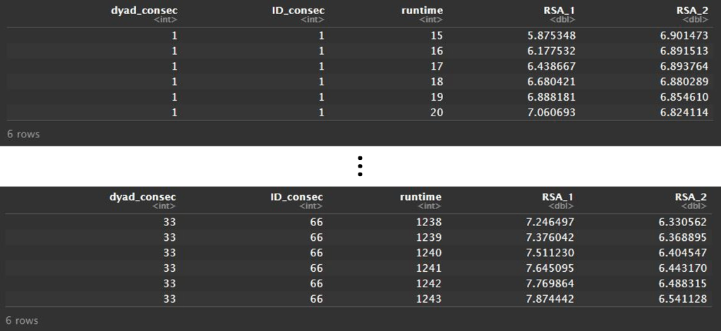
We can then plot data from one dyad to visualize an example of the patterns of RSA we see in the data. From the below plot we can see that individuals seem to have a good amount of variability which can be captured at the second by second level and are showing differences from the other member in the dyad. Interestingly we can also see that there are some moments when the two participants seem to increase in RSA at the same time and other moments when they move in opposite directions.

We can model the intra-class correlation for variation in second-by-second RSA using the rjags package in R. Variance will be partitioned into three groups. Variance which is attributed to nesting within an individual, within a dyad, and between persons. We will specify diffuse priors for mean and variance parameters as we don’t have any prior hypotheses about differences in variance parameters. In the below representation of how we are modeling our distributions, ICCi represents variation attributed to the individual, ICCd represents variation attributed to the dyad, and ICCb is the residual between dyad variation.

Now that we have our Bayesian model written out we can turn to how we are going to implement it in R using rjags. First we will grab some more information about our data so that we can successfully loop over each observation, individual, and dyad. Then we will put all of our data together into a list we will call “data” and assign it to meaningful names we will call in our rjags model.
nrofObs <- nrow(longdata) # 85,436
nrofSubjects <- length(unique(longdata$participant_1)) # 66
nrofDyads <- length(unique(longdata$dyad)) # 33

data <- list(nrofObs = nrofObs, y = longdata$RSA, ID = longdata$ID_consec, dyad = longdata$dyad_consec, nrofSubjects = nrofSubjects, nrofDyads = nrofDyads)
Like many R functions, rjags operates by parsing a model string with specific structure. Within the model we will specify each distribution beginning at the observation level and then working hierarchically upward until we reach the priors. Therefore, in the below model statement we start with specifying a normal distribution for our observation variable, centered around the observation with the variance attributed to the individual. We work our way through our levels and then finish with specifying our priors for our global mean and variance parameters and then specify that we also want to calculate ICCs for each chain.
modelString = "
model
{
for(ijk in 1 : nrofObs) {
y[ijk] ~ dnorm(mui[ID[ijk]], 1/intraVar)
}

for(jk in 1 : nrofSubjects)
mui[jk] ~ dnorm(mud[dyad[jk]], 1/dyadVar)
}

for(k in 1 : nrofDyads) {
mud[k] ~ dnorm(M, 1/interVar)
}

M ~ dnorm(0,1/100000)

intraVar    <- 1/intraPrec
intraPrec  ~ dgamma(0.001,0.001)
intraSD   <- sqrt(intraVar)

dyadVar    <- 1/dyadPrec
dyadPrec  ~ dgamma(0.001,0.001)
dyadSD   <- sqrt(dyadVar)

interSD    ~ dunif(0,1000)
interVar   <- pow(interSD,2)

# intra-class correlations
ICCi <- intraVar/(interVar + intraVar + dyadVar)
ICCd <- dyadVar/(interVar + intraVar + dyadVar)
ICCb <- interVar/(interVar + intraVar + dyadVar)

}
"
writeLines(modelString, con="ICC.txt")
We can finally move on to running our model and viewing our results! However, these types of models can take some time to run. We will indicate the parameters we are interested in following. We will then estimate the model with 1000 burn in iterations and 5000 samples from the posterior.
parameters <- c( "intraSD", "dyadSD", "interSD", "ICC", "mui", "mud", "M");
jagsModel = jags.model(file="ICC.txt",data=data,n.chains=3,n.adapt=1000)
update(jagsModel,n.iter=1000) # burn-in
codaSamples = coda.samples(jagsModel,variable.names=parameters,n.iter=5000) # samples 